Pop Art with k-means clustering
I wanted to see if I could use Machine Learning (ML) algorithms to create vibrant pop art. The goal was simple: get an image, find clusters (groups) for its pixels, and recolour.
K-Means Clustering
Out of all the different tools for clustering data, K-means Clustering is a classic. It picks k (an integer of 2 or more, e.g. 2, 3, 4, 5, 6…) random points in a data set. These random points become centroids for each cluster, i.e. the centre point of each new cluster.
Then each point is assigned one-by-one to its closest centroid and becomes part of its cluster. After this, each point is part of a cluster and we’re all done, right? Not quite. Remember that the centroids, the central points were chosen at random. The mean component of k-means clustering seeks to rectify this.
With our current clusters, we calculate the mean (average) for each cluster. Instead of our random initial centroid, we then select this as our new centroid. By doing this, we attempt to find the natural centroids in the data set, i.e. where our data is naturally clustered around.
For all our data points, we re-calculate which cluster they belong to based on our new centroids. Given our new centroid locations, we expect that some, if not many, data points will transition to new clusters. We repeat this process of re-calculating centroids and clusters until either: a) our centroids stop changing, or b) we reach a set amount of iterations.
Our future pop art
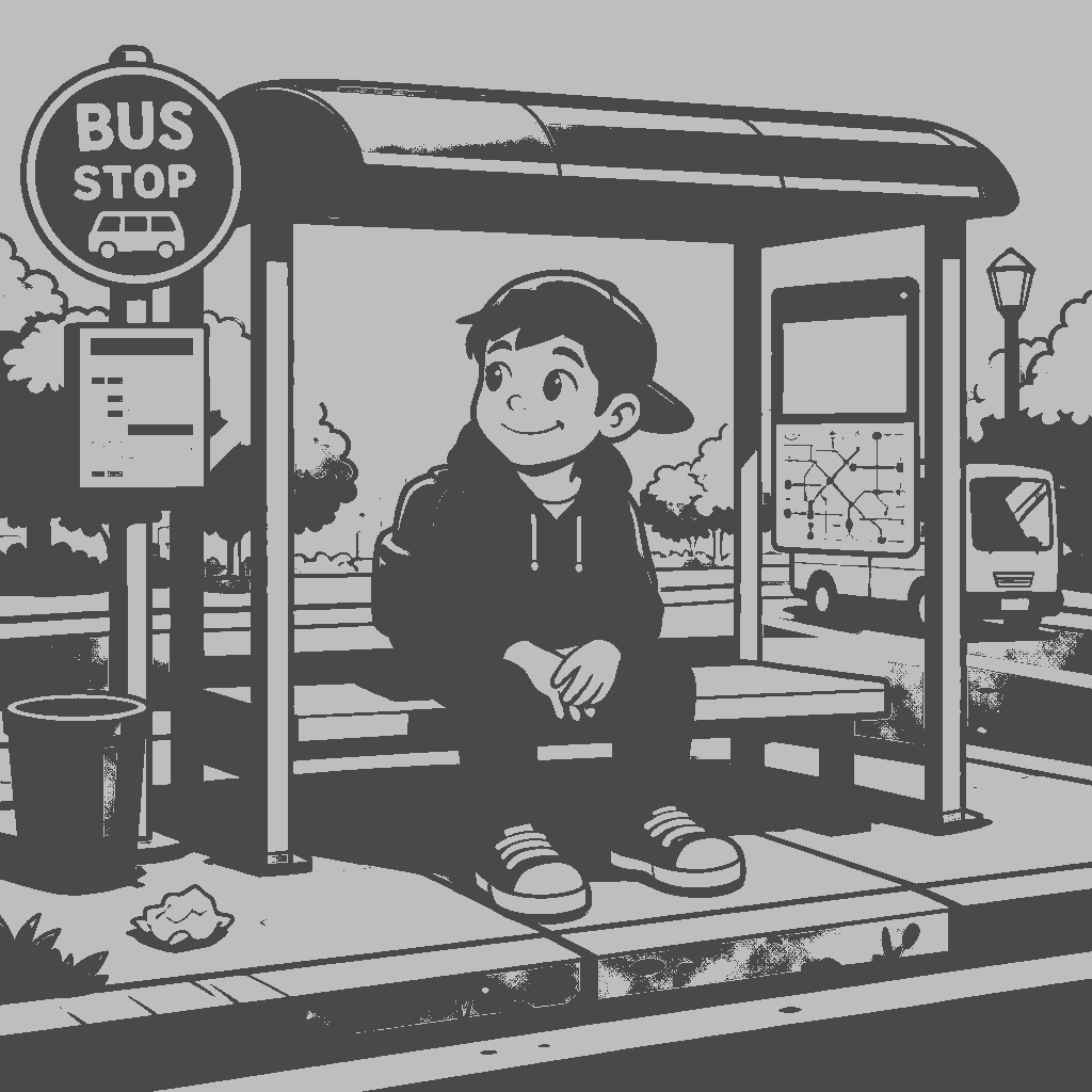
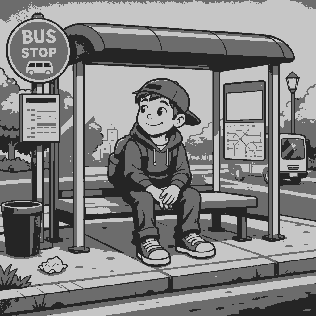
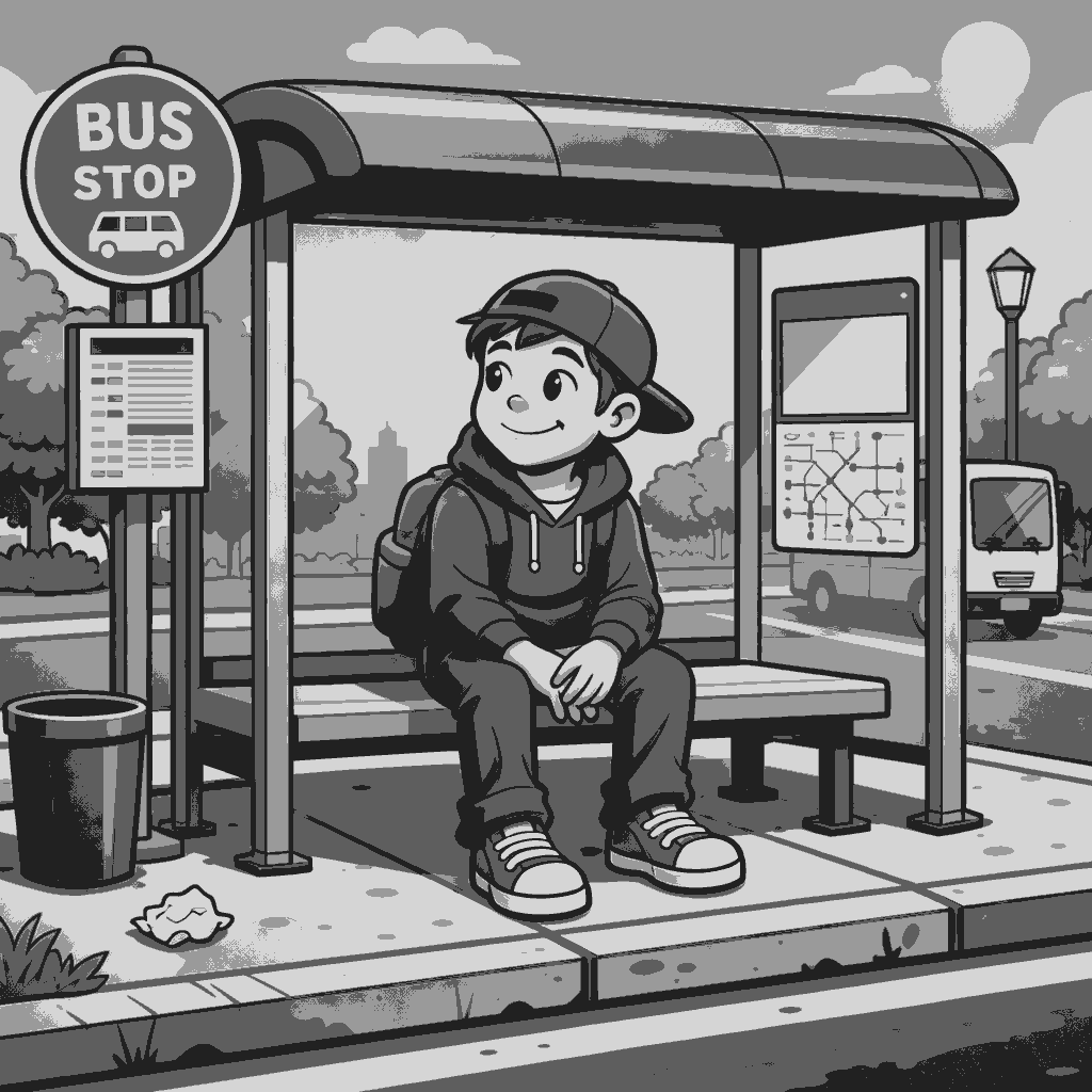
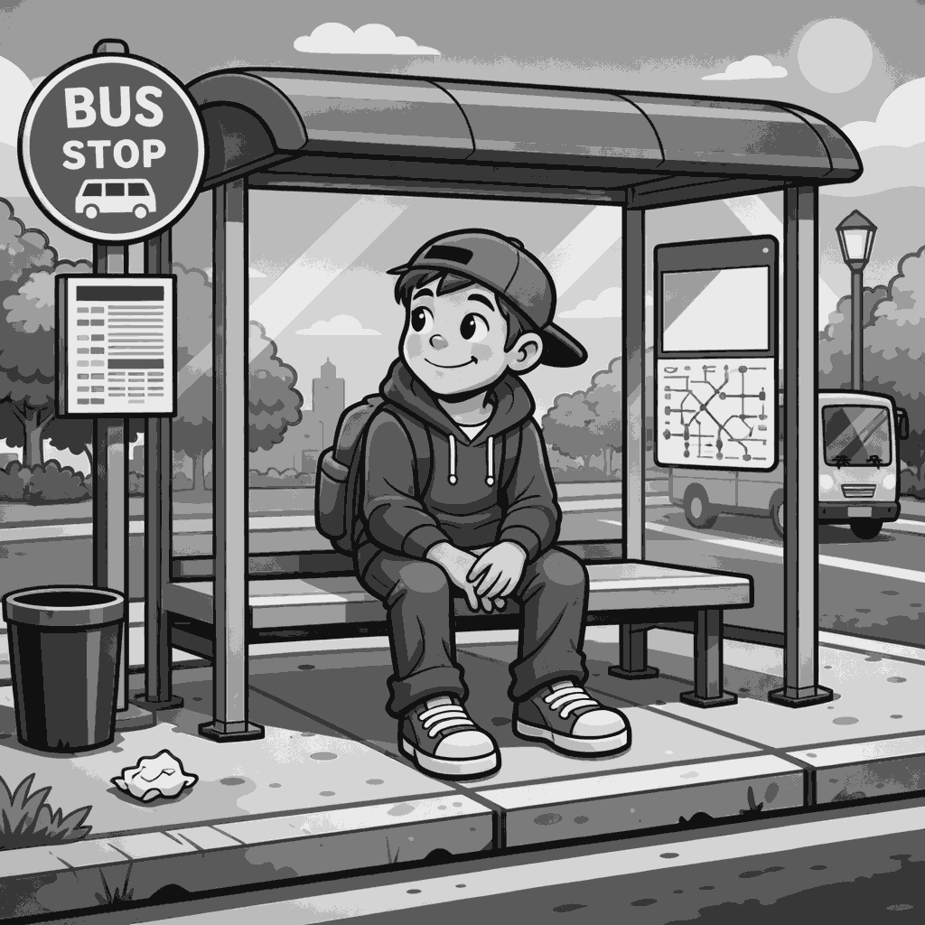
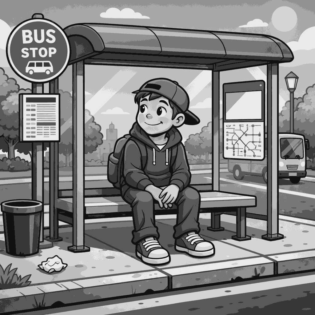
I generated this cartoon image of a boy at a bus stop. For simplicity’s sake, we’ll be using a greyscale version for our calculations.

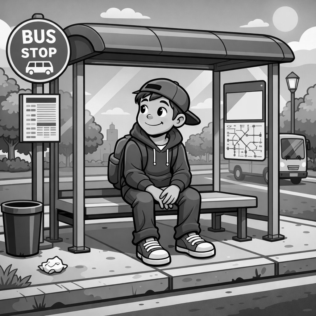
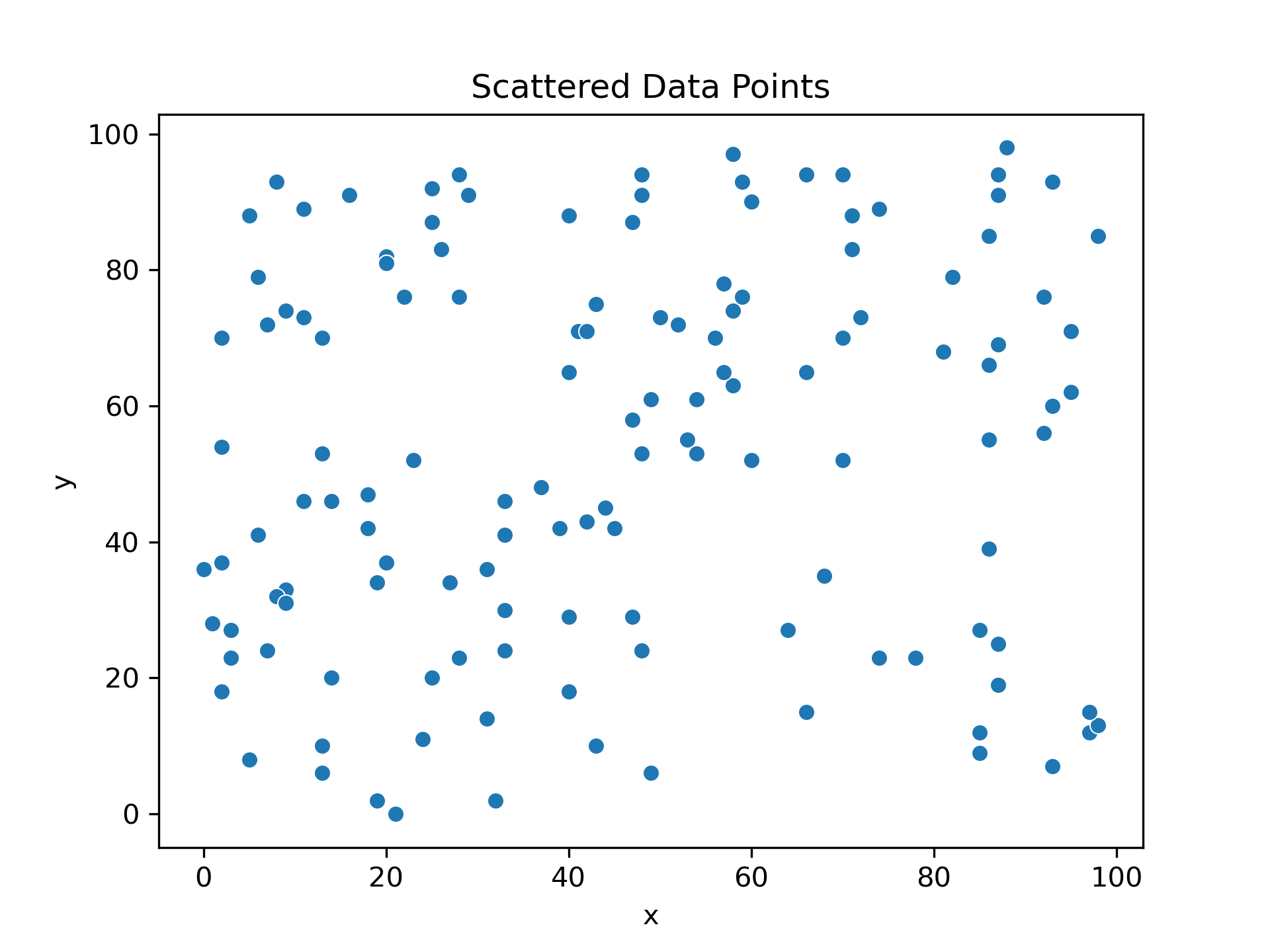
For the greyscale image, each pixel is represented by a value from 0 to 255 with 0 being pitch black and 255 being white. We can therefore use these values as our data points to cluster with K-Means.
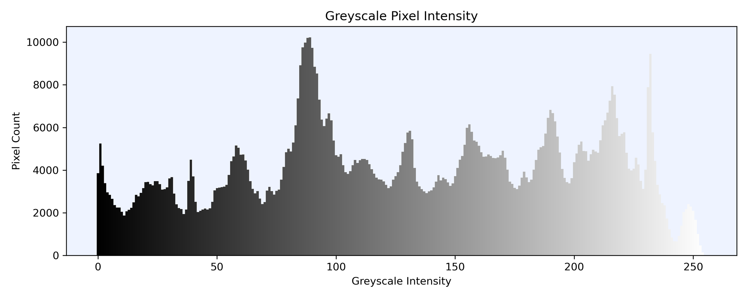
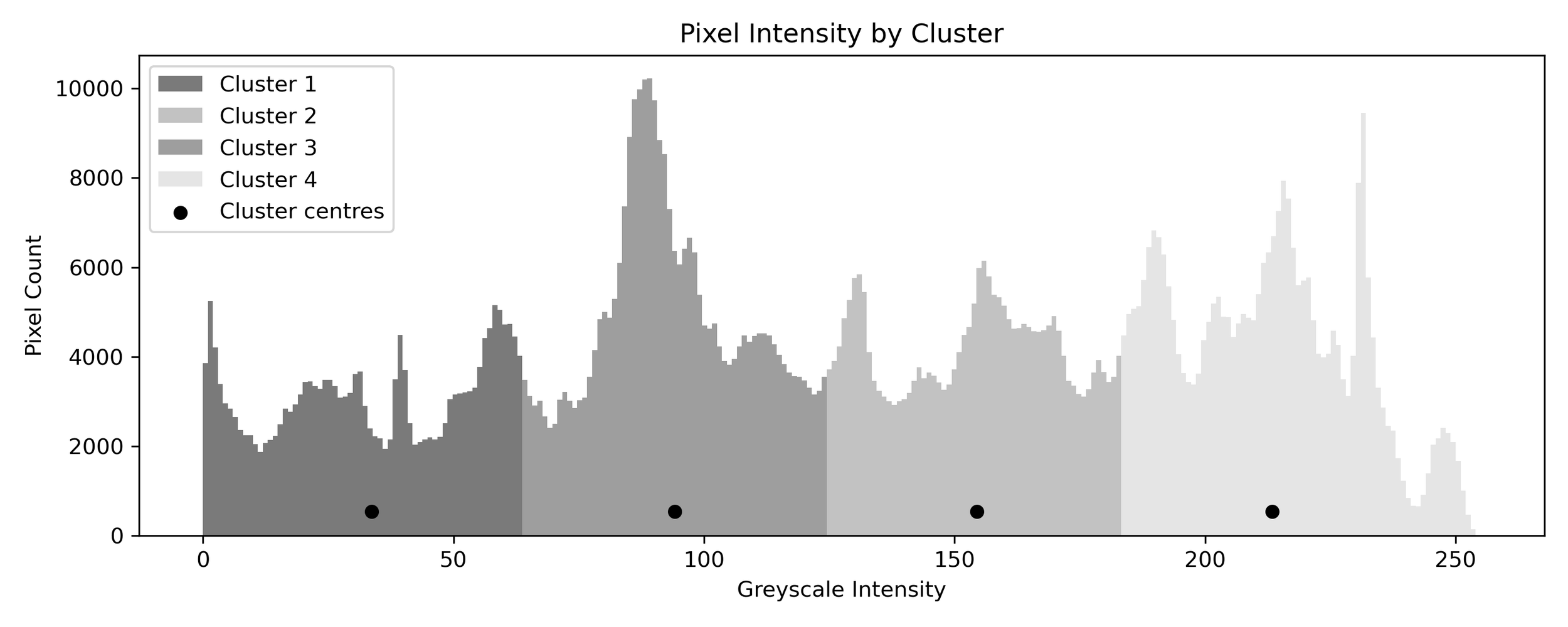
Below is a histogram of the frequency of each pixel intensity in the image from pitch black to pure white.

How many clusters?
No matter how many clusters we choose, our solution isn’t going to be perfect. With fewer clusters, we lose more information but have more stark grouping. As we increase our clusters, each cluster becomes less potentially less meaningful but we see more nuance. If we had the full 256 clusters, one for each pixel intensity, then the clusters become meaningless.
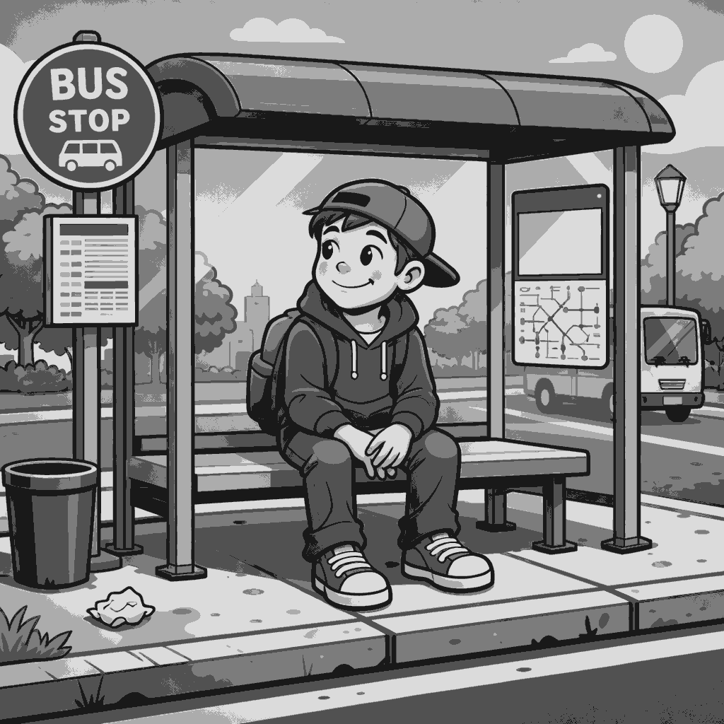
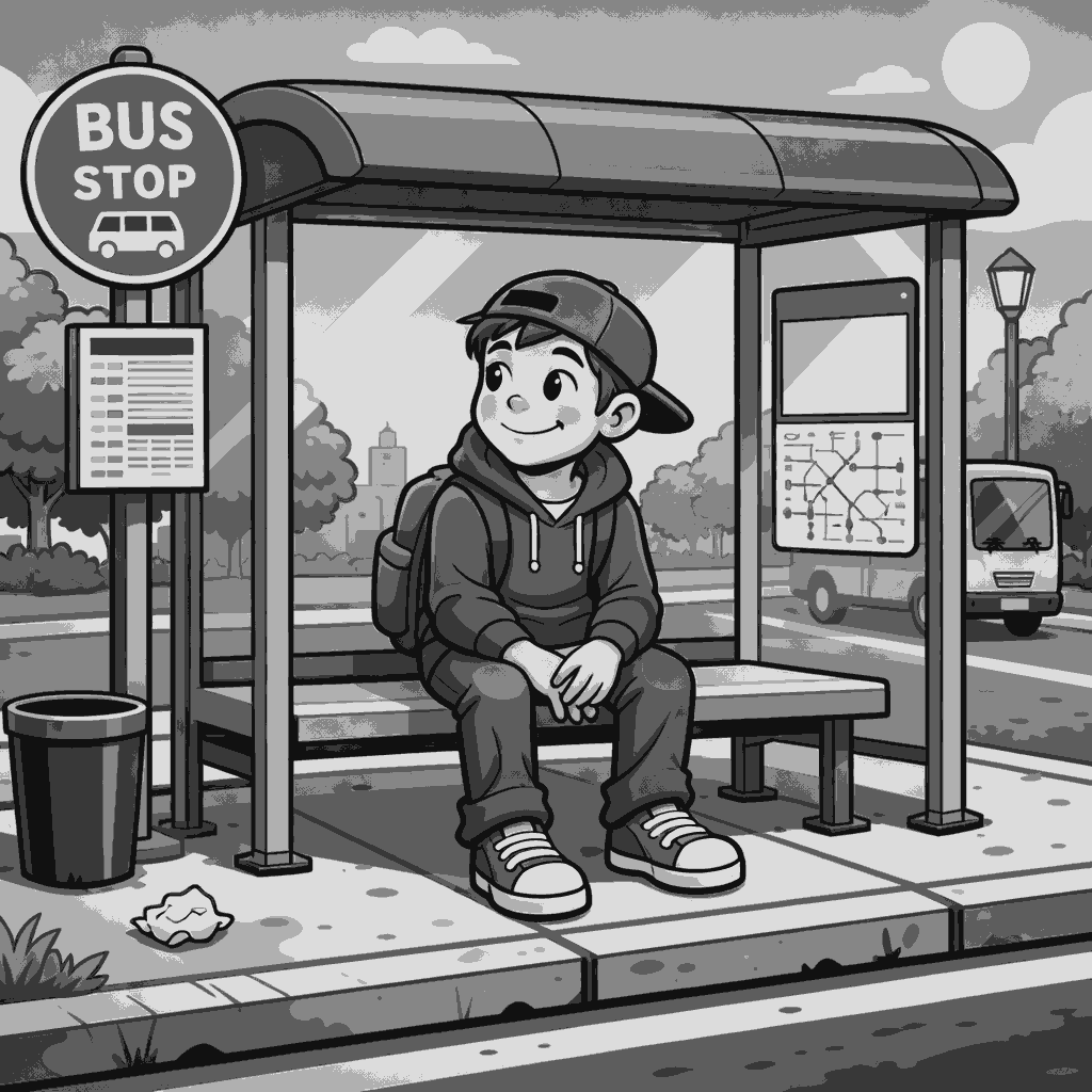
To showcase this, the following images show our greyscale image clustered into 2 to 9 clusters respectively.

To optimise our clusters, we’ll use both inertia and silhouette scores.
Inertia Score measures how condensed and tightly packed the clusters are. The lower the score, the more tightly packed they are. However, as we have more clusters this number decrease naturally, so low isn’t simply better. We’d like a distinct point where adding more clusters doesn’t give us much more gains in inertia.
Silhouette Score shows how strongly data points belong to their cluster and distinctly not to another. If many data points sit between two or more clusters groups and could nearly belong to another, then our clusters don’t capture our data well. As such, a higher silhouette score is better.
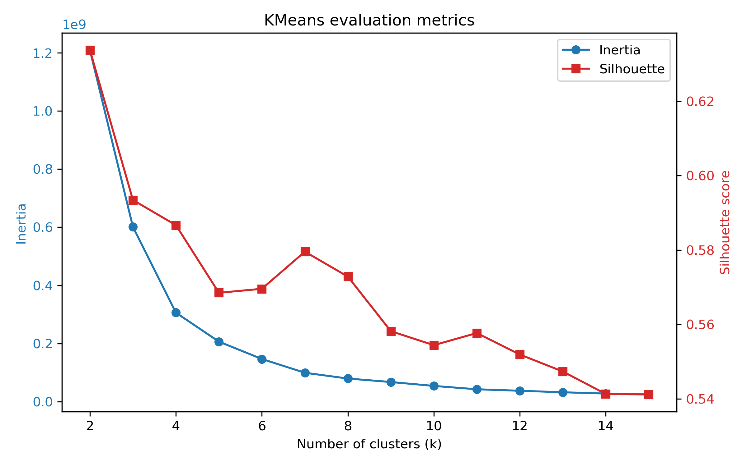
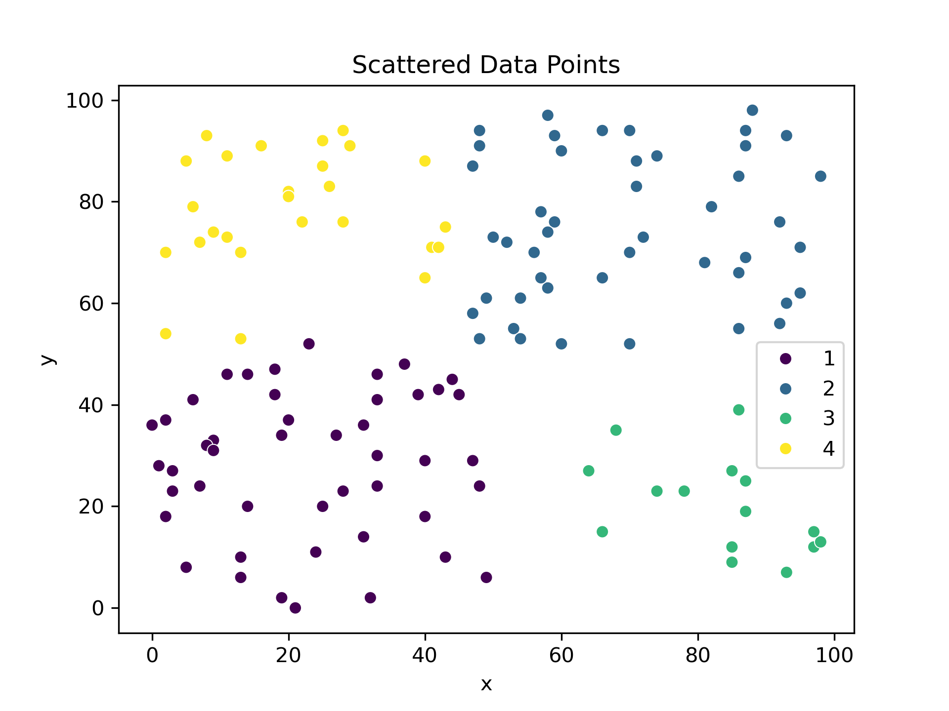
The inertia score’s rate of improvement tends to slow around k=4. Simultaneously our silhouette score drops from 4 to 5. As such, let’s move ahead with 4 clusters.
Clustering and Colouring
Recall our pixel intensity distribution from before? Here it is again, followed by the data points split into 4 clusters and then recoloured with some pop art colours.
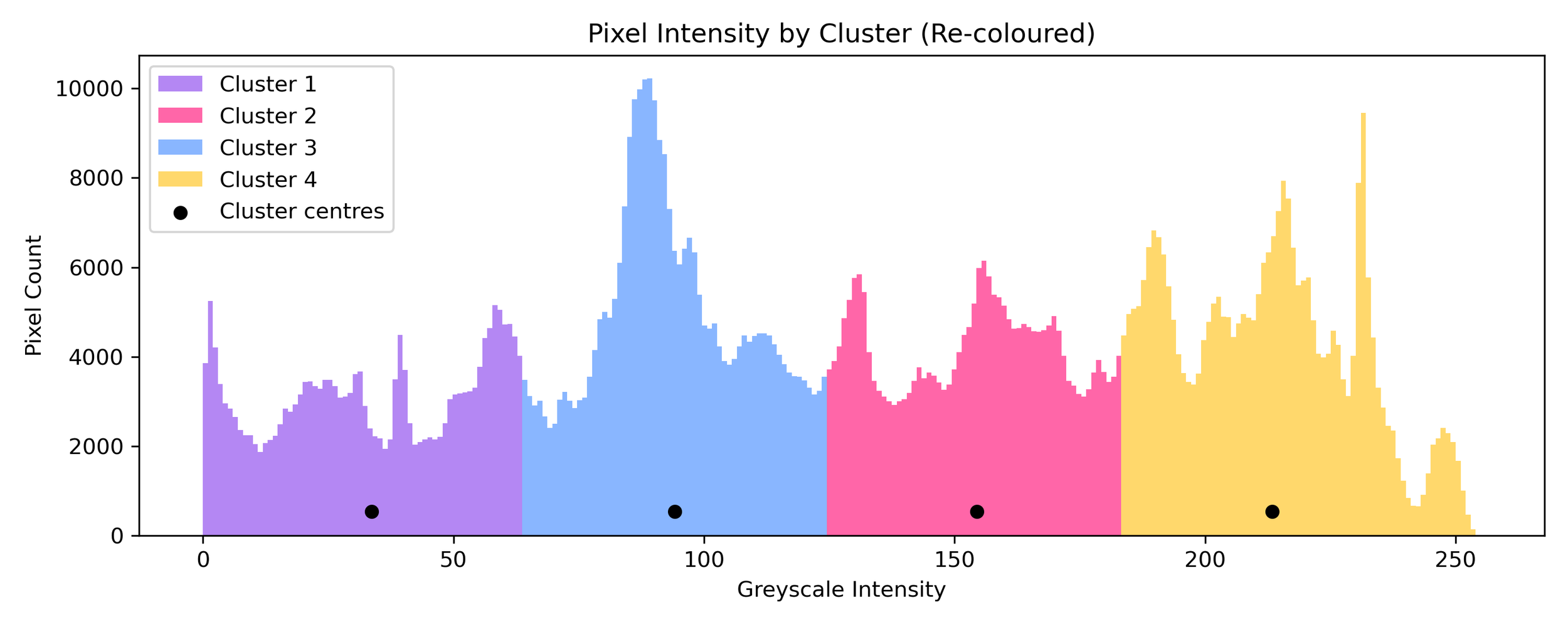
Now, we can return to our original greyscale image and for each pixel find the cluster it belongs to and recolour it accordingly.
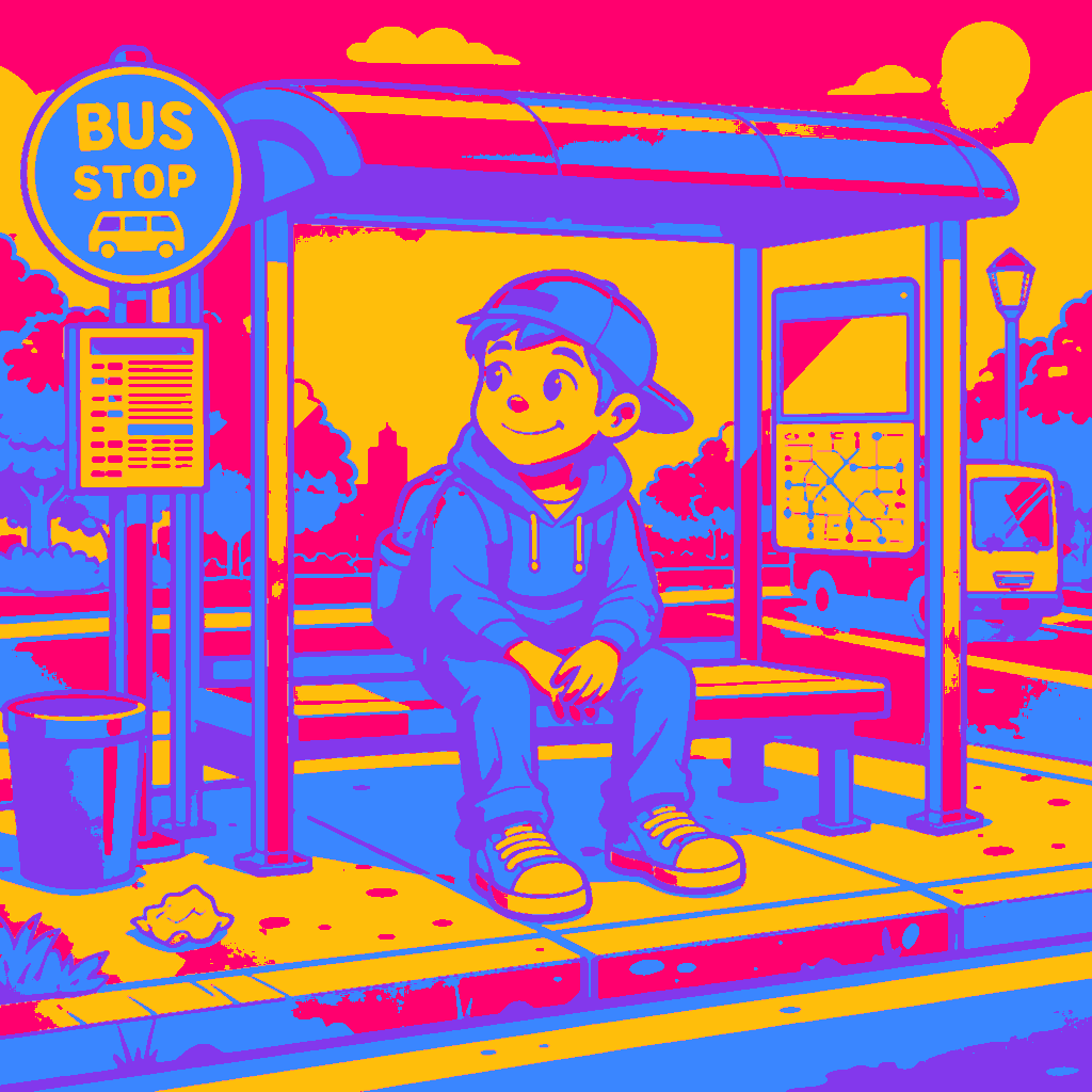
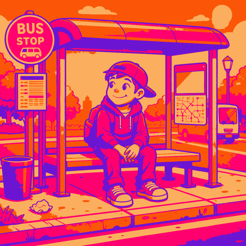
With some slight image smoothing, our final result looks like this.
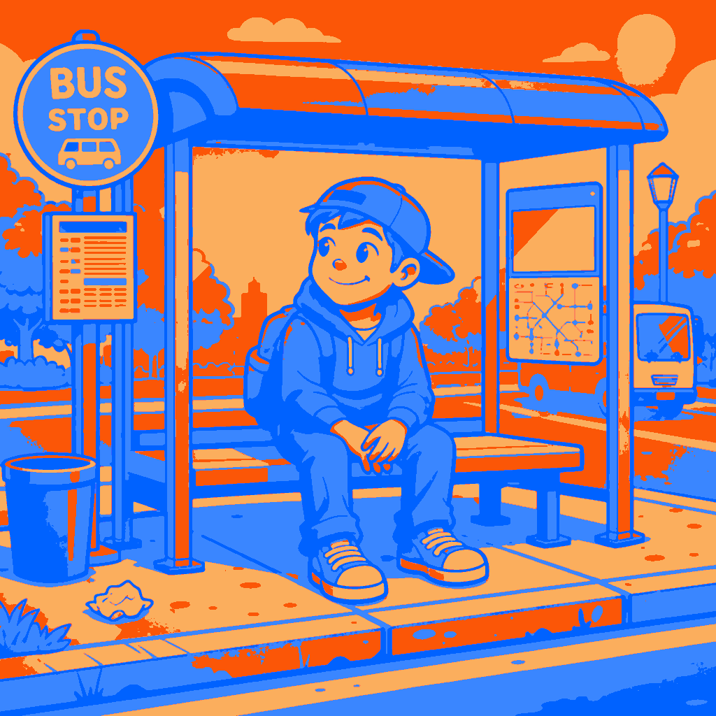
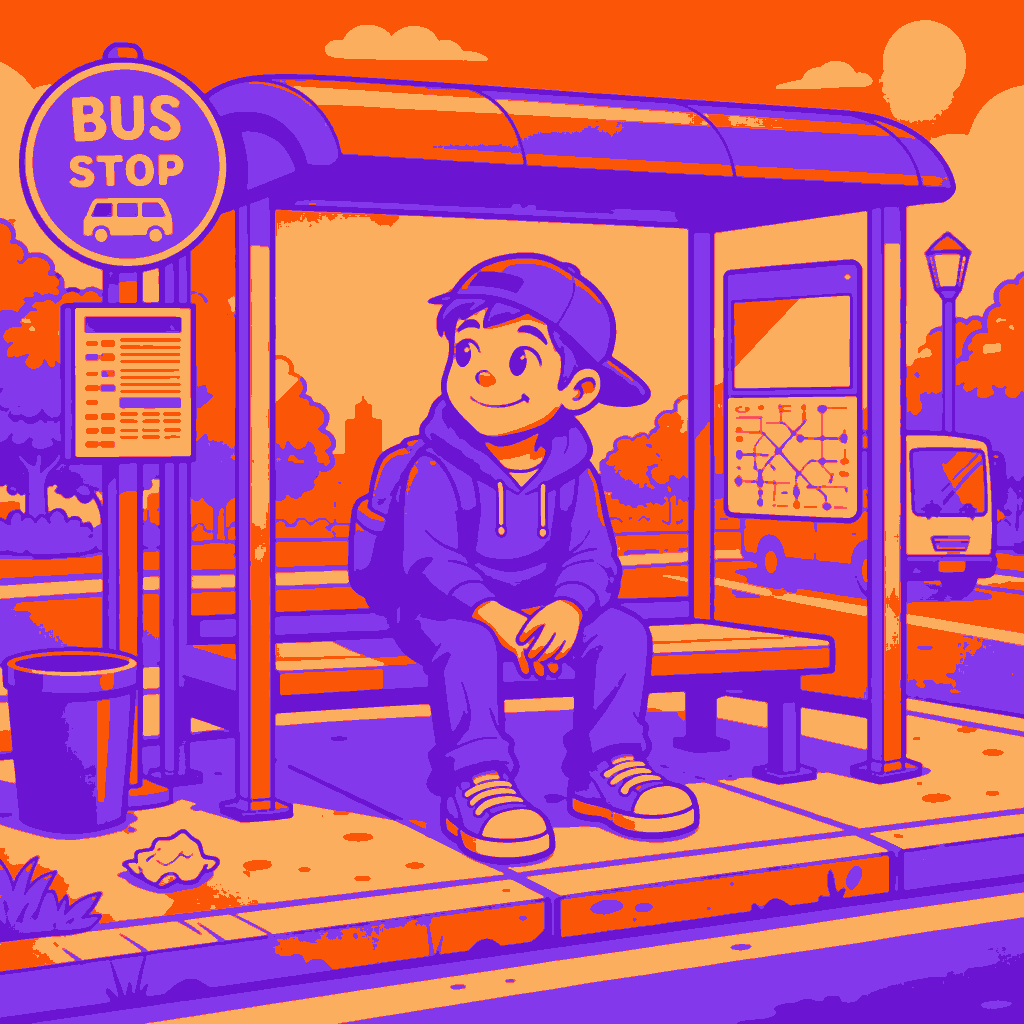
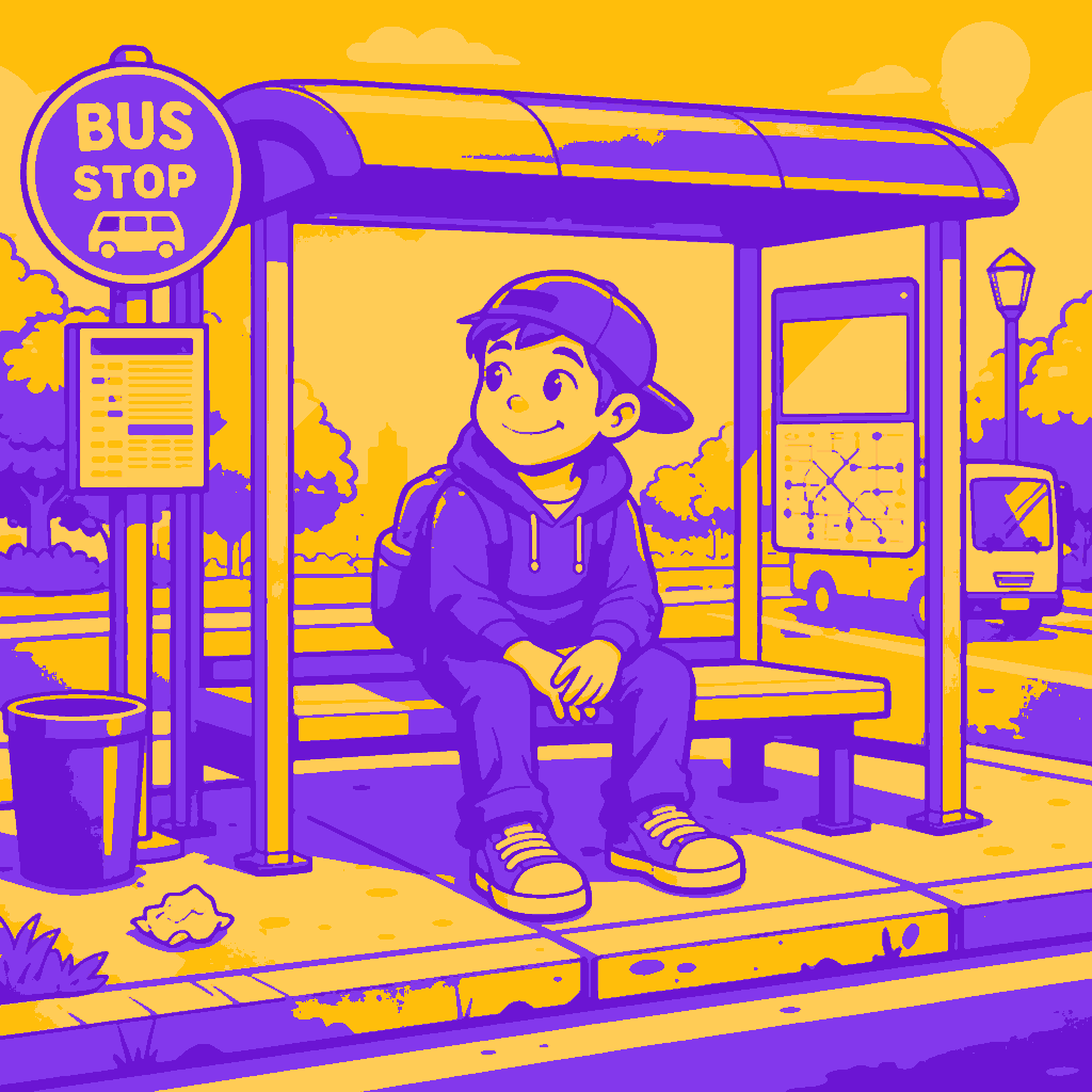
Here are a few more variations.
Photos don’t seem to work as well due to their rich and nuanced colour palette. Nonetheless, here are some cute puppies now as pop art.
As a fun note, I’ve included an example of what happens dark colours are accidentally replaced with lighter ones. My deepest apologies.
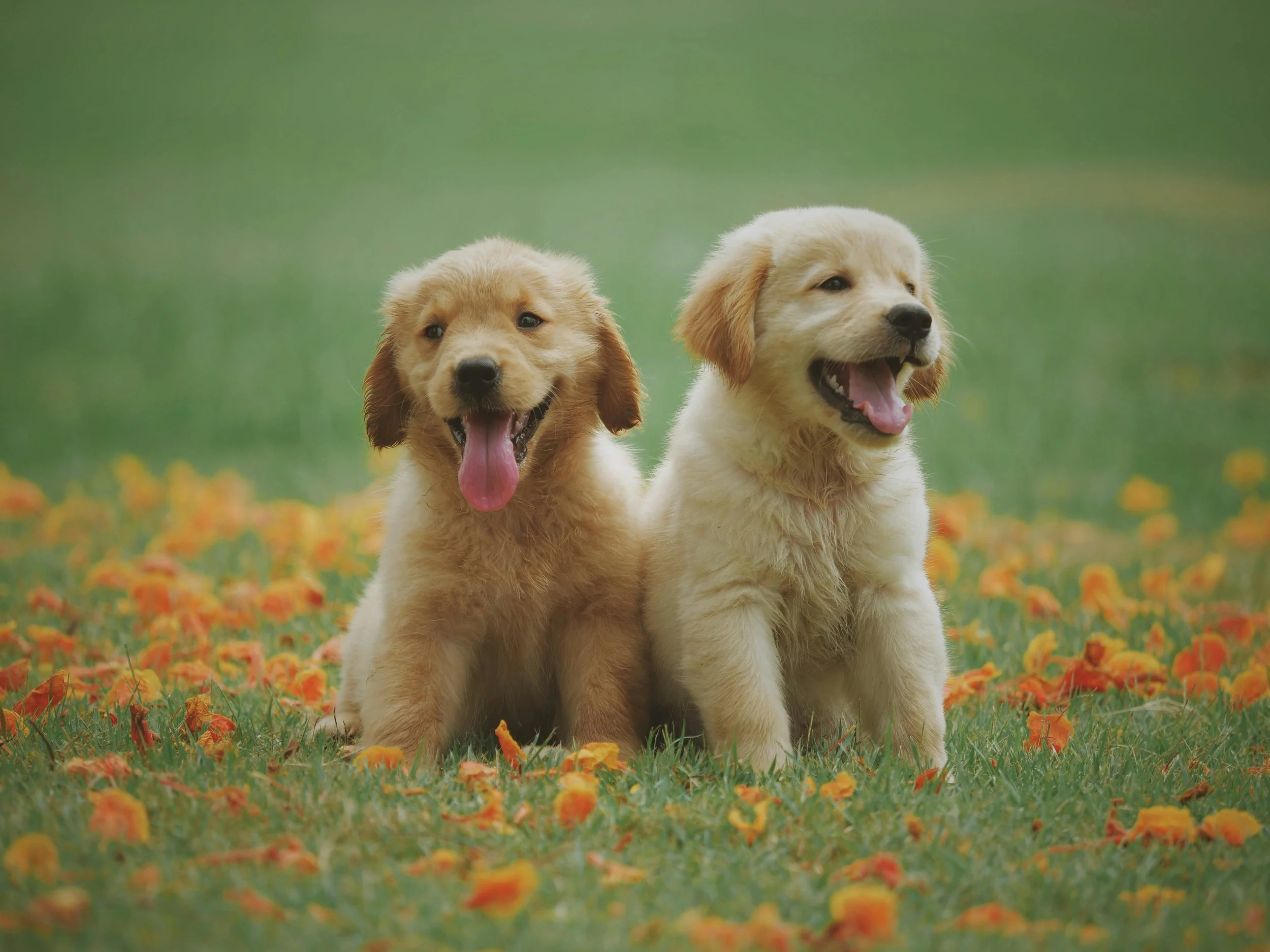
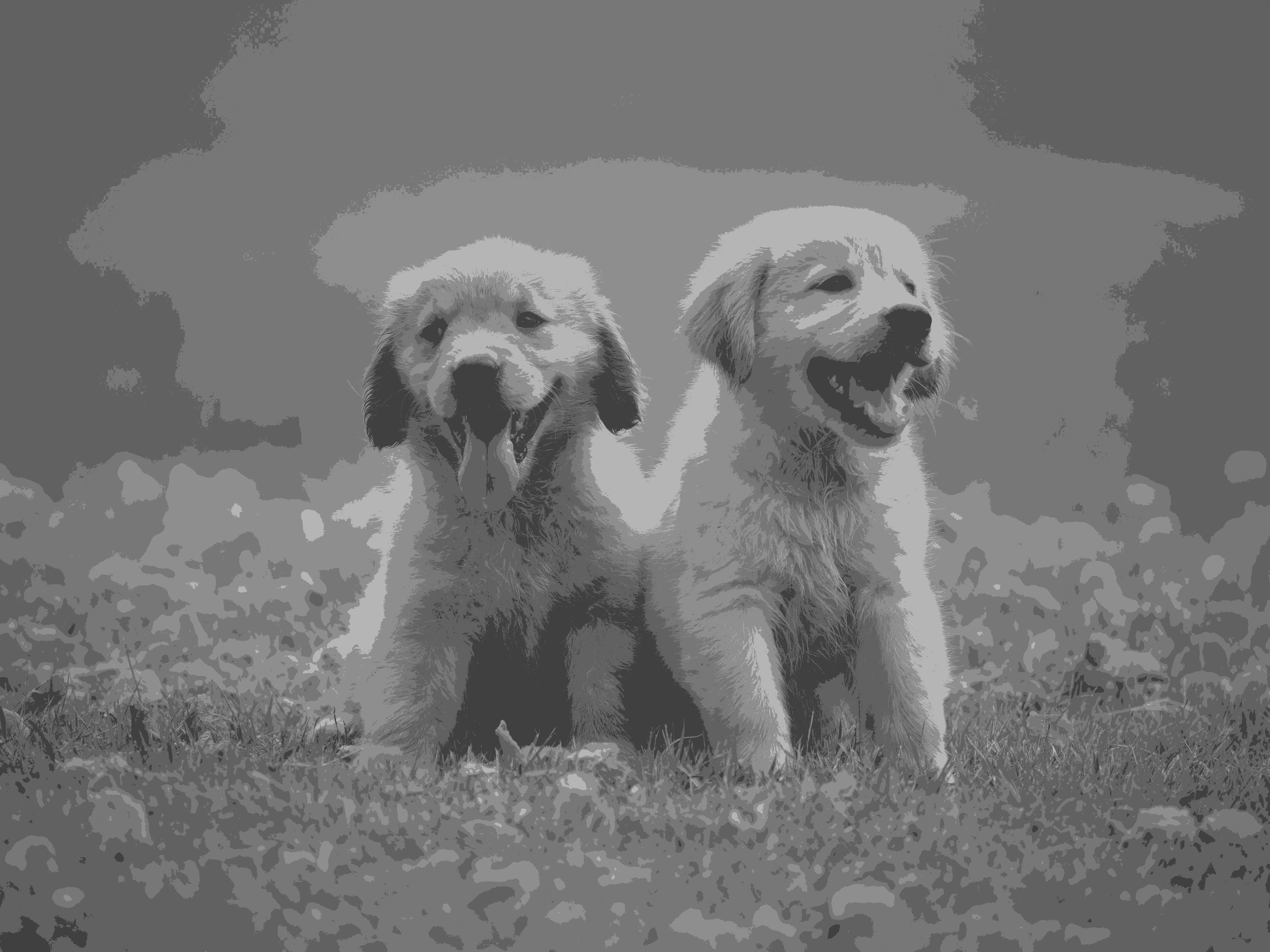
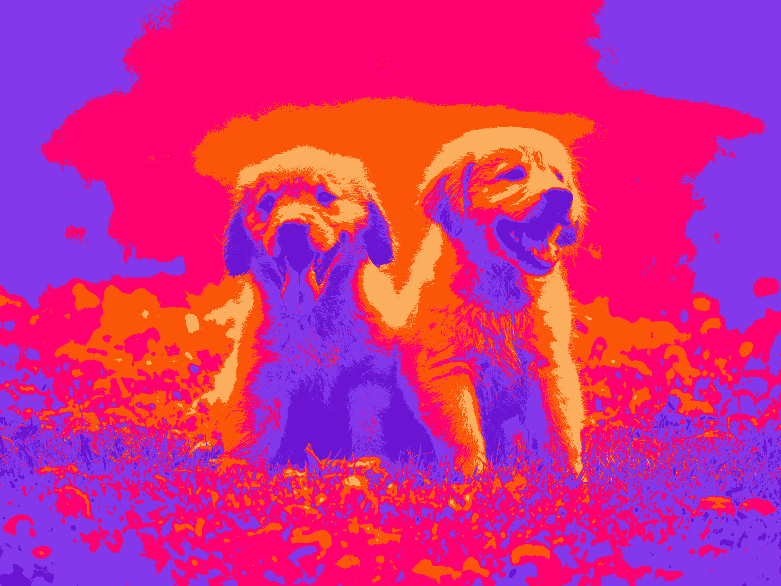
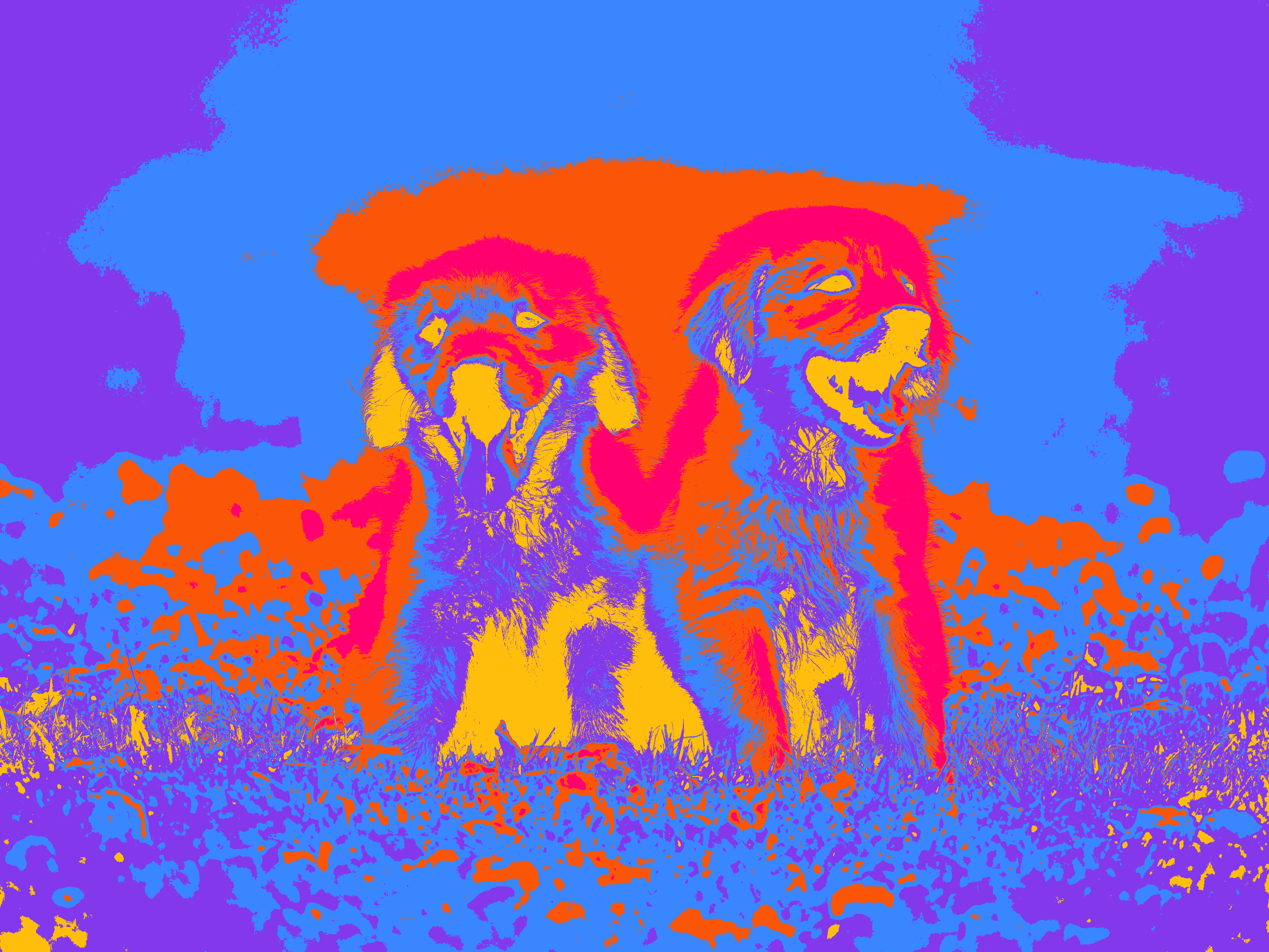
Image courtesy of Chevanon Photography: https://www.pexels.com/photo/2-1108099/